This lesson gives you some tricks for viewing and interpreting Treatment Optimization Model (TOM) outputs. It uses the outputs generated in the Treatment Optimization Model lesson, the four vector, 12 grid output items, and the Ideal Landscape themes. You do not necessarily have to use the small Happy data for this lesson, you can use outputs from a different landscape, just be sure you have all the output themes. This lesson assumes you have some experience using FlamMap to modify legends, changing units, and displaying different themes. If you do not have these skills, first complete the Basic Lessons. If you need to review these skills you can click on the blue links in this lesson as you need to, which refer to the online help system.
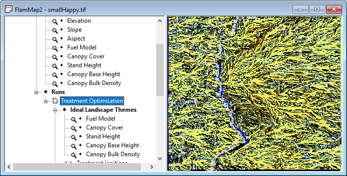
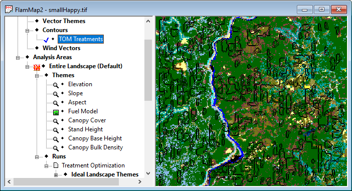
After completing the run, close the "Run:" dialog, and expand ![]() Treatment Optimization item in the "Tree" pane your project window will look like this.
Treatment Optimization item in the "Tree" pane your project window will look like this.
Some of the outputs should seem similar to those created by a MTT run. The ![]() ♦Max Spread Direction and
♦Max Spread Direction and ![]() ♦Elliptical Dimension output items are designed as inputs for other applications and will not be discussed in this lesson. You can find out more on these grids by clicking on the above links. The
♦Elliptical Dimension output items are designed as inputs for other applications and will not be discussed in this lesson. You can find out more on these grids by clicking on the above links. The ![]() ♦Rate of Spread and
♦Rate of Spread and ![]() ♦Fireline Intensity items are identical to those generated in an MTT run and are created to give a pre-treatment baseline for these two fire behavior characteristics. The output items that begin with the word "Treat" or "TOM" are based on the treated landscape created by TOM.
♦Fireline Intensity items are identical to those generated in an MTT run and are created to give a pre-treatment baseline for these two fire behavior characteristics. The output items that begin with the word "Treat" or "TOM" are based on the treated landscape created by TOM.
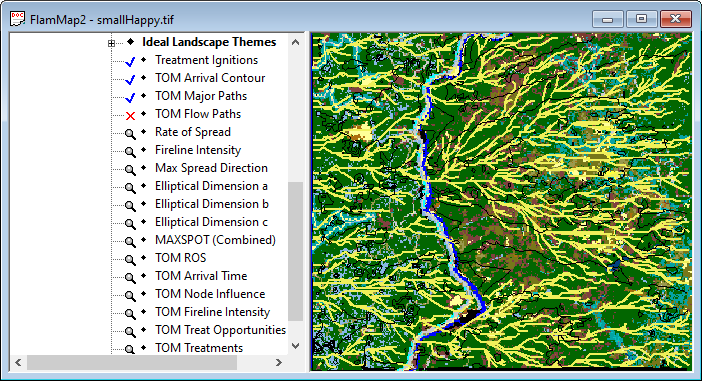
The ![]() ♦ Treatment Ignitions item is simply the display of the ignition file you specified on the Treatment Optimization Model tab.
♦ Treatment Ignitions item is simply the display of the ignition file you specified on the Treatment Optimization Model tab.
Turn off (by double-clicking) the ![]() ♦TOM Flow Paths
item to make viewing easier. This theme can be confusing except for viewing when zoomed in close since it shows the path of the fire from the ignition to EVERY one of the nodes.
♦TOM Flow Paths
item to make viewing easier. This theme can be confusing except for viewing when zoomed in close since it shows the path of the fire from the ignition to EVERY one of the nodes.
The ![]() ♦TOM Major Paths
and
♦TOM Major Paths
and ![]() ♦TOM Flow Paths
items are very similar to the paths discussed in the MTT tutorial. There are several differences in this lesson,
♦TOM Flow Paths
items are very similar to the paths discussed in the MTT tutorial. There are several differences in this lesson,
the paths cover the entire landscape since there is no time period specified for a TOM run,
these paths originate from the west border of the landscape, and
they are based on the treated landscape created by TOM.
Turn off the ![]() ♦TOM Major Paths
and
♦TOM Major Paths
and ![]() ♦Treatment Ignitions
items to make viewing easier. Don't forget you can turn on any vector or contour item simply by double-clicking, feel free to do this at any time in this lesson as you continue to explore TOM outputs.
♦Treatment Ignitions
items to make viewing easier. Don't forget you can turn on any vector or contour item simply by double-clicking, feel free to do this at any time in this lesson as you continue to explore TOM outputs.
The ![]() ♦TOM Arrival Contour
is simply a contour of the
♦TOM Arrival Contour
is simply a contour of the ![]() ♦ TOM Arrival Time grid item. The outputs shown may be different from yours for several reasons, the stochastic nature of simulated spotting, the legend properties, or input differences.
♦ TOM Arrival Time grid item. The outputs shown may be different from yours for several reasons, the stochastic nature of simulated spotting, the legend properties, or input differences.

Notice that the non-burnable river bottom significantly slowed the spread of the simulated fire.
Now turn off the ![]() ♦TOM Arrival Contour
item.
♦TOM Arrival Contour
item.
The ![]() ♦TOM Treatments is a display of the treatments suggested by TOM.
♦TOM Treatments is a display of the treatments suggested by TOM.
Remember the treatments are just the values specified in the ideal landscape. You may want to think of the ![]() ♦TOM Treatments as the "cookie cutter" which cuts the treatments from the ideal landscape (smallHappyIdeal.tif) and pastes them onto the original landscape (smallHappy.tif). These are the locations that had the most impact on delaying or altering fire spread under the simulated conditions and Treatment Fraction.
♦TOM Treatments as the "cookie cutter" which cuts the treatments from the ideal landscape (smallHappyIdeal.tif) and pastes them onto the original landscape (smallHappy.tif). These are the locations that had the most impact on delaying or altering fire spread under the simulated conditions and Treatment Fraction.
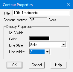
Since FlamMap can only display one grid theme at a time it can be awkward (likely impossible) to remember where TOM placed treatments when viewing the fire behavior outputs. Here is a simple trick to "convert" the ![]() ♦TOM Treatments into a vector theme.
♦TOM Treatments into a vector theme.
|
|
1. Make 2. Right click the 3. Enter 0.5 in the Contour Interval: text box. 4. Click the OK button to close the "Contouring" dialog. |
Contouring the ![]() ♦TOM Treatments creates a new
♦Auxiliary Themes > ♦Contour >
♦TOM Treatments creates a new
♦Auxiliary Themes > ♦Contour >
![]() ♦TOM Treatments
contour item. Unfortunately the contouring function creates a double line around each of the treatment areas with the inner most line being the most accurate. Now select the
♦TOM Treatments
contour item. Unfortunately the contouring function creates a double line around each of the treatment areas with the inner most line being the most accurate. Now select the ![]() ♦Fuel Model item as your active grid.
♦Fuel Model item as your active grid.
Notice that this new contour is in the ♦Auxiliary Themes part of the "Tree" pane.
|
|
To make the treatments more visible by right-clicking on the Increase the line width to "2". Leave the |
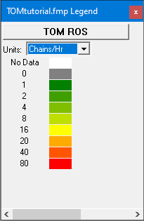
The ![]() ♦Rate of Spread and
♦Rate of Spread and ![]() ♦TOM ROS grids are shown below. They use the same default Chains/hour legend.
♦TOM ROS grids are shown below. They use the same default Chains/hour legend.
The ![]() ♦Rate of Spread grid is the result of a MTT run for the ignition smallWestIgnition.shp on the original landscape (smallHappy.tif). The
♦Rate of Spread grid is the result of a MTT run for the ignition smallWestIgnition.shp on the original landscape (smallHappy.tif). The ![]() ♦TOM ROS grid is the rate of spread with the treatments shown in the
♦TOM ROS grid is the rate of spread with the treatments shown in the ![]() ♦TOM Treatments theme. Remember, these are rates of spread along the paths shown above. They are NOT the rates of spread you would see from the Fire Behavior Options tab outputs.
♦TOM Treatments theme. Remember, these are rates of spread along the paths shown above. They are NOT the rates of spread you would see from the Fire Behavior Options tab outputs.
|
|
|
|
Pre treatment Rate of Spread grid. |
Post treatment Treat ROS grid. |
|
|
As you can see by the legend the green colors are the slower and the post treatment ROS grid ( More importantly notice the significant reduction of spread rates OUTSIDE of the treatment areas. This is where TOM is different from other methods of identifying fuel treatments, TOM optimizes the treatment locations to affect the entire landscape. More information on the Treatment Optimization Model can be found in the help system Technical Topics. |
Similar to the rate of spread grids, pre and post treatment fireline intensity grids are also created. The pre treatment ![]() ♦Fireline Intensity grid is shown on the left below while the post treatment
♦Fireline Intensity grid is shown on the left below while the post treatment ![]() ♦Treat FLI is on the right. The two grids have the same default legend, Fireline Intensity kW/m.
♦Treat FLI is on the right. The two grids have the same default legend, Fireline Intensity kW/m.
|
|
|
|
Pre treatment Fireline Intensity grid. |
Post treatment Treat FLI grid. |
As with the ROS grids, notice the post treatment reduction in fireline intensity outside the treated areas. Because TOM places units to increase the amount of non-head spread (i.e. backing and flanking) over the entire landscape, the fireline intensity is also reduced over the entire area.
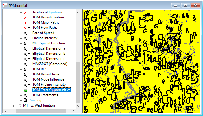
The ![]() ♦Treatment Opportunities grid simply compares the two landscapes (smallHappyIdeal.tif) and (smallHappy.tif) in this case. It is very handy for evaluating your ideal landscape before running TOM. First notice that all the TOM proposed treatments occur in the yellow areas.
♦Treatment Opportunities grid simply compares the two landscapes (smallHappyIdeal.tif) and (smallHappy.tif) in this case. It is very handy for evaluating your ideal landscape before running TOM. First notice that all the TOM proposed treatments occur in the yellow areas.
|
|
The This is why TOM only selects treatment in the positive areas, there is no benefit (fire behavior wise) for treating if the rate of spread cannot be reduced. |
When testing ideal landscapes the areas of positive benefit should be several times the expected treatment fraction to allow TOM to choose the best treatment placement. Usually a positive value for at least 50% of the landscape is necessary to achieve good results with TOM, but more is always better.
The last TOM output is the ![]() ♦Treat Node Influence grid. Basically it is a measure of the contribution of a cell to the overall spread of the simulated fire across the landscape. The darker color indicates a larger contribution. In a TOM run it is calculated for the post treatment landscape.
♦Treat Node Influence grid. Basically it is a measure of the contribution of a cell to the overall spread of the simulated fire across the landscape. The darker color indicates a larger contribution. In a TOM run it is calculated for the post treatment landscape.

The ![]() ♦Treat Major Paths
item is derived from the
♦Treat Major Paths
item is derived from the ![]() ♦Treat Node Influence grid, this is why the major paths overlay the higher value cells.
♦Treat Node Influence grid, this is why the major paths overlay the higher value cells.
Notice how some of the major paths go through the treatments and some skirt the edges. The TOM algorithm is designs treatments so that the simulated fire takes just as long to go around the treatment as it does to go through it. This assures the maximum effect of the allowed treatment fraction.
The Treatment Optimization Model is a complex tool dealing with the relatively new concept of designing fuel treatments for the landscape as a whole, instead of individual stands. These lessons are just an introduction, so before using this tool for designing operational fuel treatments practice with the MTT fire growth and TOM methods on familiar landscapes. Read and refer to the help system Technical Topics and reference literature to help ensure that your analysis is correct.
Related Topics